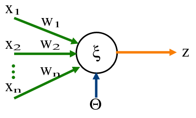
The human brain is an intricate web of billions of interconnected neurons that allow us to process information, make decisions, and perform complex tasks. This remarkable ability has inspired the creation of artificial neurons, like the perceptron, which mimic biological neurons in a simpler form. These artificial neurons are the building blocks of Artificial Intelligence (AI), enabling machines to learn and evolve.

What is a Perceptron?

Imagine a single neuron,a tiny but essential unit in the vast neural network of your brain. It activates when it receives signals, processes them, and decides what to do next. Similarly, a perceptron is the most basic computational unit of a neural network. Its invention by Frank Rosenblatt in the late 1950s laid the foundation for modern AI.

Think of it as a decision-making machine. It takes inputs, applies some rules, and generates an output. Despite its simplicity, the perceptron unlocks the doorway to understanding more complex systems.

Breaking Down the Perceptron

To understand a perceptron, let’s peek inside its mind. It starts with a set of inputs, let’s call them \( x_1, x_2, x_3 \)and their corresponding weights \( w_1, w_2, w_3 \). These weights reflect the importance of each input. The perceptron combines these inputs by multiplying each with its weight and summing them up.

For example, consider:

- Inputs: \( x_1 = 1, x_2 = 2, x_3 = 3 \)
- Weights: \( w_1 = 0.5, w_2 = 1, w_3 = -1 \)

The perceptron computes the weighted sum:
\[ (x_1 \times w_1) + (x_2 \times w_2) + (x_3 \times w_3) \] Plugging in the values:
\[ (1 \times 0.5) + (2 \times 1) + (3 \times -1) = 0.5 + 2 - 3 = -0.5 \]

Next, the perceptron applies an activation function, which determines the output. If we use a linear activation function (i.e., the value remains as it is), the output here is (-0.5). This output can help classify data, for example, negative values could indicate Type A, and positive values Type B.

The Magic of Learning

Here’s where the magic happens. A perceptron isn’t just about calculating outputs, it’s about learning. It adjusts its weights based on errors in its predictions, using a process called backpropagation.

When we train a perceptron, we provide it with a dataset of known inputs and outputs (a training set). The perceptron compares its predictions to the actual outcomes, calculates the error, and tweaks its weights. This iterative process, guided by gradient descent, helps the perceptron improve over time, enabling it to make accurate predictions even for unseen data.

The magic starts with backpropagation, where the perceptron “learns” by iteratively adjusting its weights to minimize errors.

If you’re curious about gradient descent, I highly recommend this video series by 3Blue1Brown, which explains it beautifully.

Final Thoughts

As the perceptron learns, it converges to a solution, a line that separates the data into distinct categories. While perceptrons are excellent for solving linear problems, they have their limitations. For instance, they can’t handle non-linear problems.

Modern neural networks, however, build upon the perceptron. By combining multiple perceptrons across layers and introducing advanced neuron types, they tackle a vast array of complex problems. From identifying faces to predicting stock prices, these networks are transforming the world as we know it.

Starting with a perceptron is like learning the alphabet before writing a novel, it’s simple yet foundational. And for me, it was the perfect entry point into the incredible world of Machine Learning.

Abhinav Thorat

Research Scientist, AI Researcher and astrophile. Avid learner with diverse interest in coding, machine learning along with topics like psychology, anthropology, philosophy & astrophysics. 6+ years of experience working in multinational corporations.